R0
= ![]() lxmx
.
lxmx
.
Introduction: Demographic processes such as births, deaths, immigration, and emigration, are those that affect the size and composition of a population. The timing of these processes also plays a critical role; a population with high juvenile mortality will have a very different structure from a population with high mortality in the post- reproductive years. Life tables are tables of data on survivorship and fecundity of individuals within a population. A standard method is to collect data on a cohort, or group of individuals all born in the same time period. Life tables constructed this way are called cohort life tables. They can then be used to determine age- or stage-specific fecundity and mortality rates, survivorship, and basic reproductive rates, which in turn can be compared from cohort to cohort enabling an analysis of their annual variation.
Importance: Understanding these demographic processes and how they affect populations is a central concern of population and conservation biologists.
Question: How do life tables help us to understand the demography of a population?
Variables:
| x | life stage or age class |
| ax | total number of individuals observed at each stage or class |
| lx | proportion of original number of individuals surviving to the next stage or class; survivorship |
| dx | proportion of original number of individuals dying during each stage or class; mortality |
| qx | mortality rate for each stage or class |
| kx | "killing power;" |
| Fx | total fecundity, or reproductive output of entire population, for each stage or class |
| mx | individual fecundity, or mean reproductive output, for each stage or class |
| lxmx | number of offspring produced per original individual during each stage or class; product of survival and reproduction |
| R0 | basic reproductive rate |
Methods: Once the life stages or age classes have been defined and the number of individuals in each have been counted, we can begin calculating values for the other variables of the life table. Survivorship (lx) is a standardized value for the number of individuals at each stage. The first survivorship value entered in any life table (l0) is always 1.0; one hundred percent of the individuals are observed at the first stage. Subsequent values for lx are calculated by dividing the number of individuals observed at a given stage by the original number of individuals (ax/a0). The mortality (dx) at each stage can then be calculated by subtracting survivorship values (lx ó lx+1). The mortality rate (qx) for each stage gives an idea of the intensity of mortality at that stage; qx is calculated by dividing mortality by survivorship (dx/lx). The "killing power" (kx) also reflects the intensity of mortality, but kx values can be summed across stages. Killing power is defined as log10(ax/ax+1) ( which = log10ax ó log10ax+1), and can also be calculated with lx values in place of ax values.
The next three variables (Fx, mx, and lxmx) are part of the life tableís fecundity schedule. Fx and mx are simply counts of the total number of offspring produced and the mean number of offspring produced per individual at each stage, respectively. Fx can be used to calculate the basic reproductive rate, R0, but the more common calculation uses the formula
R0
= ![]() lxmx
.
lxmx
.
which is the sum of the number of offspring produced per original individual during each stage.
The following data were collected for an annual plant,
Phlox
drummondii (after Leverich & Levin 1979, in Begon et al.
1996):
|
|
|
|
|
|
|
|
|
|
|
|
|
|
|
|
|
|
|
|
|
|
|
|
|
|
|
|
|
|
|
|
|
|
|
|
|
|
|
|
|
|
|
|
|
|
|
|
|
|
|
|
|
|
|
|
|
|
|
|
|
|
|
|
|
|
|
|
|
|
|
|
|
|
|
|
|
|
|
|
|
|
|
|
|
|
|
|
|
|
|
|
|
|
|
|
|
|
|
|
|
|
|
|
|
|
|
|
|
|
|
|
|
|
|
|
|
|
|
|
|
|
|
|
|
|
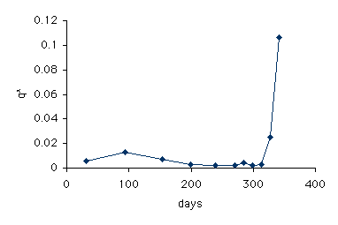
Notice that plants were not reproductive until the 292-306 day age-class. We can graph the daily mortality rate (qx) to see at which points in its life history P. drummondii is most vulnerable.

Interpretation: Phlox plants appear to be most vulnerable (excluding death from "old age") in the first three age classes, with a peak in the second one (63-124 days). If conservation of this species were needed, we would know to expend our efforts during these three time intervals to maximize the success of this population. Based on these data, however, the basic reproductive rate of this population (R0) was 2.41; the population increased by a factor of 2.4. At least when these data were collected, the population was not in any danger of decreasing in size.
Conclusions: Life table data can provide much insight into the demographics of a population. Quantifying age-specific birth and death rates enables us to discern patterns and make predictions about the growth or decline of populations in the future.
Additional question:
1. Calculate the killing power (kx) for this plant using the ax values. For what age class is killing power the highest?
Source: Begon, M., J. L. Harper, and C. R. Townsend. 1996. Ecology: Individuals, Populations, and Communities, 3rd edition. Blackwell Science Ltd. Cambridge, MA.
copyright 1999 M. Beals, L. Gross, S. Harrell